Reliability in the Lincoln-Petersen Method of Estimating Population Size

The Lincoln-Petersen method allows you to estimate the size of a population based on two separate observations of that population. For example, we might be interested in the global population of the eastern imperial eagle. In that case, the number that we’re after is the population size, N. If N = 5K, that means there are 5K eastern imperial eagles in the world. But counting every single eastern imperial eagle in the world is hard: that is why we are trying to estimate it.

The detection probability p describes how likely we are to observe each individual. So if we went into the field and observed 50 eastern imperial eagles, that means p = 50 ÷ 5,000 = 1%. We usually don’t know this either, for if we did we would also know N.

Finally, n is the number of individuals that were captured and marked on the first visit, K is the number of individuals captured on the second visit and k is the number of individuals captured on the second visit that were also marked from the first visit. The Lincoln-Petersen method relies on the fact that n ÷ N = k ÷ K, in other words that the proportion of marked individuals is (in expectation) identical both in the whole population and in any randomly selected subset of it. Say for example that we marked n = 500 eastern imperial eagles on our first visit; if we then also capture K = 500 on the second visit and if k = 50 of those were marked, we would estimate a population of N = n × K ÷ k = 500 × 500 ÷ 50 = 5,000 eastern imperial eagles. (For a more arcane but perhaps also thorough description of this method, see my other post.)

The detection probability p could be high in the first observation and low in the second one or vice versa and still not adversely affect the reliability of the estimates because it doesn’t change the equation: n ÷ N = k ÷ K. It doesn’t matter if you detect more or fewer individuals in the second visit, because the proportion of them that is marked will still equal the proportion that is marked in the whole population. Though actually, in some cases it does matter, as we shall see shortly …

Estimating Body Counts #

In the previous posts I described first how an official in the fictional Kingdom of Tamego went about estimating killings in a civil war in that country and then how one can program a Bayesian model for estimating population sizes based on this sort of capture-recapture data. In the course of making the model – or rather extending a model that Marc Kéry and Michael Schaub described in Bayesian Population Analysis using WinBUGS and that Hiroki Itô translated into Stan – in the course of so extending, I made many simulated-data experiments for which the model (and the Lincoln-Petersen method) produced pretty bad estimates.

This kind of mystified me. In some experiments, the method produced very accurate estimations, but in others they were wildly off the mark. For a while I thought this was because the Lincoln-Petersen method did not handle data with variable detection probability well. I noticed that when I halved the detection probability for one of the observations (so that the probability of detecting an individual was higher or lower on the second visit than on the first, for example because a different method of observation was used), then estimations got much less accurate. But as mentioned above, that was a red herring. The reason that observations were worse was that I saw too few marked individuals in the second visit, which introduced a lot of noise in the model.

Experiments #

This is the kind the experiment I ran, in R code:

f <- function(N, p) {
  n <- rbinom(1, size = N, prob = p)
  K <- rbinom(1, size = N, prob = p)
  k <- rbinom(1, size = K, prob = n/N)
  return(n*(K/k))
}

This function does the following. First it simulates the number of individuals caught in the first visit n, based on population size N and detection probability p. Then it simulates the number of individuals caught in the second visit K and the subset of those that were marked from the first visit k. Finally it returns the Lincoln-Petersen estimate.

> f(500, .1)
[1] 258.375

Right off the bat, with a population size of 500 and a detection probability of ten percent, we get a weak estimate, about half of the true population. But if we increase the detection probability to 50%, we get a much more accurate estimation:

> f(500, .5)
[1] 489.8571

However, then we have to capture half of the population. That seems like a lot. What if we try to estimate a larger population with the ten percent detection probability?

> f(5000, .1)
[1] 4068.119

This, too, is better – about one fifth off from the true population. What if we have a really large population but a low detection probability?

> f(50000, .01)
[1] 29701.75

That’s a pretty bad estimate, once again off by nearly half. In general, it seems that estimates improve when either population size or detection probability (or both of these) increase. Specifically, estimates seem to be unreliable when k – the number of recaptured individuals that were also marked – is small. We can modify our function to return k in addition to N:

f <- function(N, p) {
  n <- rbinom(1, size = N, prob = p)
  K <- rbinom(1, size = N, prob = p)
  k <- rbinom(1, size = K, prob = n/N)
  return(c(k, n*(K/k)))
}

Then we see that k is in single digits for the first and last experiments – the two that saw bad estimates:

> f(500, .1)
[1]   8.000 258.375
> f(500, .5)
[1] 126.0000 489.8571
> f(5000, .1)
[1]   59.000 4068.119
> f(50000, .01)
[1]     8.00 29701.75

Take for example the last one, with a population of 50K and a detection probability of one percent. With k = 10 instead of k = 8, the estimate would drop to 23,761 (-5,940); with k = 6 instead of k = 8, the estimate grows to 39,602 (+9,901). These are really large changes in estimates from just detecting a couple more or fewer marked individuals. In other words, some combinations of population sizes and detection probabilities are much more volatile than others.

We can visualise this volatility by making a bunch of counterfactual experiments. For any given set of simulated data, we can calculate how far off the correct estimate we would be for k = 1, k = 2, k = 3 and so on. If the range of k values that give us a good estimate is really narrow, we can’t trust the results of a Lincoln-Petersen estimate, because normal variation will cause the estimate to fluctuate wildly. Here are these counterfactuals for each of the four experiments I ran above:

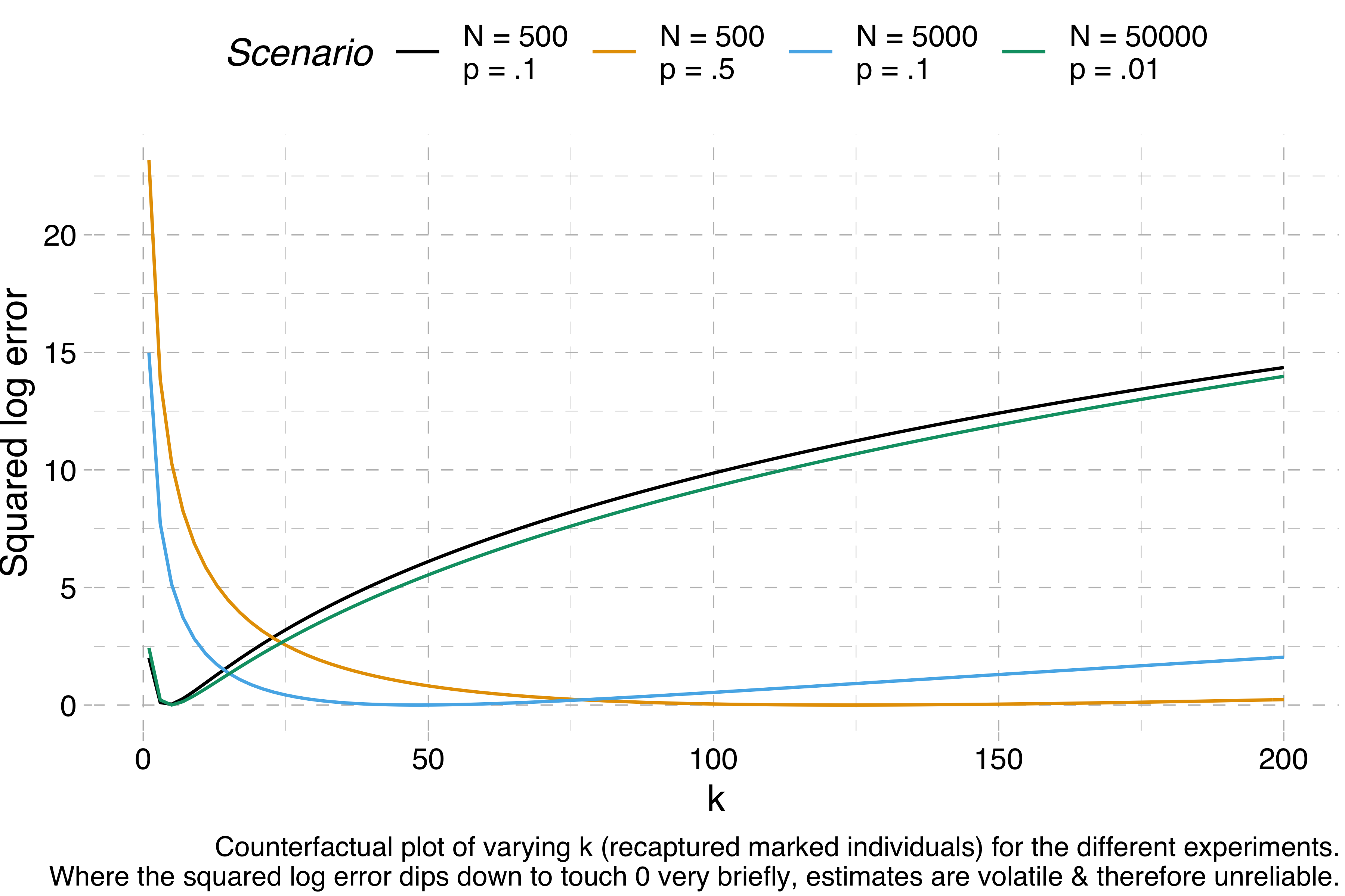
The y-axis shows the squared log error – when this is 0, the estimation is perfect, but the higher it is, the further away the estimation is from the target. We can see that N = 500, p = 10% and N = 50,000, p = 1% are both estimated correctly for a narrow range of values of k – the squared log error dips down quickly before quickly rising again – whereas the other two scenarios, for which correct estimations require much higher values of k, give us much more room for error.

If I am correct about this, then I think the Lincoln-Petersen method alone does not provide good estimations of sparse populations. The eastern imperial eagle really does have an estimated population of ~5K individuals. So if you have p = 1%, that is, if you have a detection probability of one percent, then the closest you could get to the true population count is by recapturing exactly one marked individual (though really you’d expect to recapture exactly one half of a marked individual, because 5,000 × .01² = .5). If you find two, the error is already bad. If you find none, you’re suddenly dividing by zero. We’d need to have a detection probability of 10% or more to start getting really reliable estimates. That seems like a pretty tall order for such a sparsely populated species (though I’m sure population ecologists have ways of dealing with this problem).

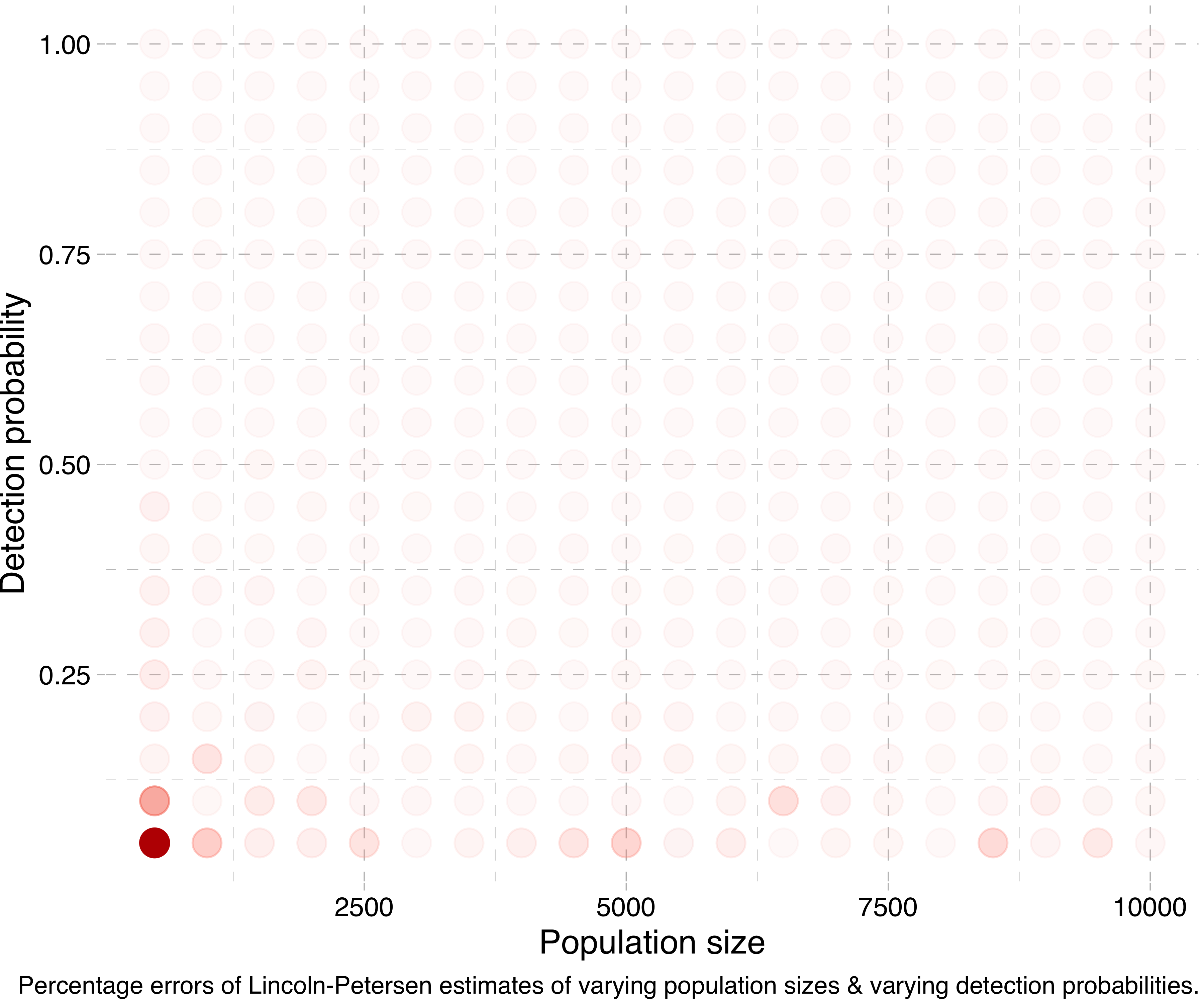
Another way of visualising this is by running a lot of simulations for different population sizes and detection probabilities, calculating the Lincoln-Petersen estimates and seeing how far off they are from the true population sizes. (Actually, in the following experiments I run the simulation for each combination five times and take the mean of the estimates, in order to smooth things out.) Doing this, we get a plot like this:

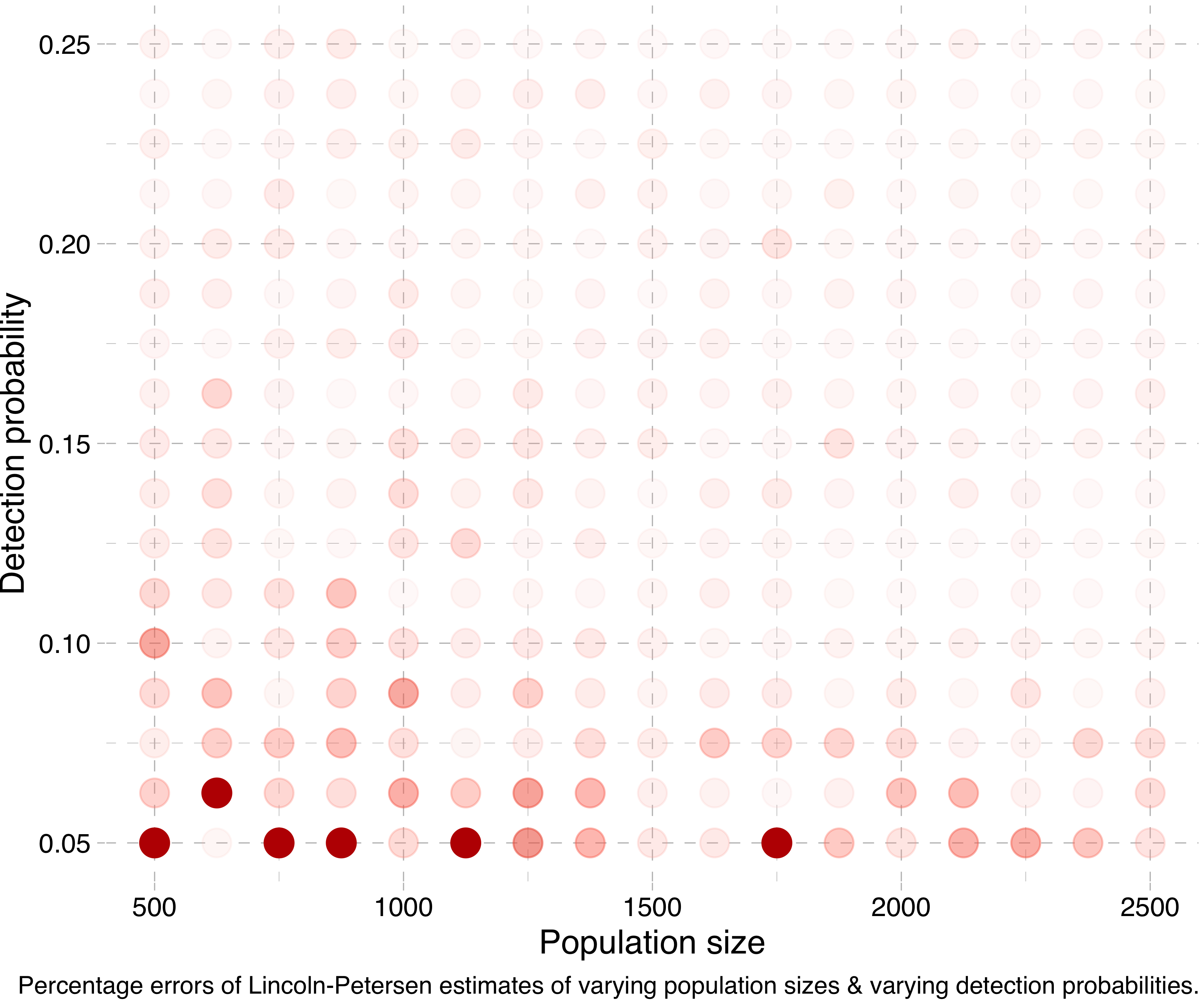
Or at a smaller scale:

To sum up, the Lincoln-Petersen method does not provide reliable estimates for small sample sizes. I suppose I could have saved you the trouble of reading this whole thing by just writing that. But sometimes only the long and tortuous path brings us to a point of real vantage.

Like this post? Subscribe via RSS or join the email newsletter: