Bayesian Modelling of Simulated Data from the Kingdom of Tamego

If a kindly man asked you in a job interview or on a first date or god forbid during a colonoscopy or something if you were interested in hearing about the loves and sorrows of his imaginary friends, you, a person of no mean sense, would nine out of ten times think he was crazy or, worse still, socially inept. Yet here you are reading about my own imaginary kingdom, with its made-up name, made-up queen and made-up war. I have nothing but praise for you, dear reader.

The previous post in this series was a fairy tale of sorts that related the story of an official in the Kingdom of Tamego who, having been tasked with estimating how many subjects were killed in a dreadful civil war, realised that the answer to his problem and the key to estimating population sizes with the kind of information that he had were so-called capture-recapture methods. In a breathtakingly ironic twist, he did not get the chance to bring his insight back to his queen but died instead a pauper in a remote district of the kingdom. We, however, can pick up and carry his torch into the modern age.

In this post I will describe a Bayesian model for estimating killings by each faction in the simulated Kingdom of Tamego data. The model is based on one described by Marc Kéry and Michael Schaub in Bayesian Population Analysis using WinBUGS and translated by Hiroki Itô into Stan. I was pointed to this technique by (and in general received a great deal of help from) folks at the Stan forums.^[1] I have only made a few minor modifications. But before I get to those, it is worth going over how Kéry & Schaub’s original model works.

Remember, the problem is this. We have three factions – the Angu rebels, the king’s forces and the Zid separatists. Each of these took part in a devastating civil war and killed a certain number of people during it. Information on these killings comes from two sources: the official military records and a census carried out some years after the civil war had ended. Each of these lists contains the name and birthplace of the slain, so we know how many people are mentioned in both of these sources. That will be important later.

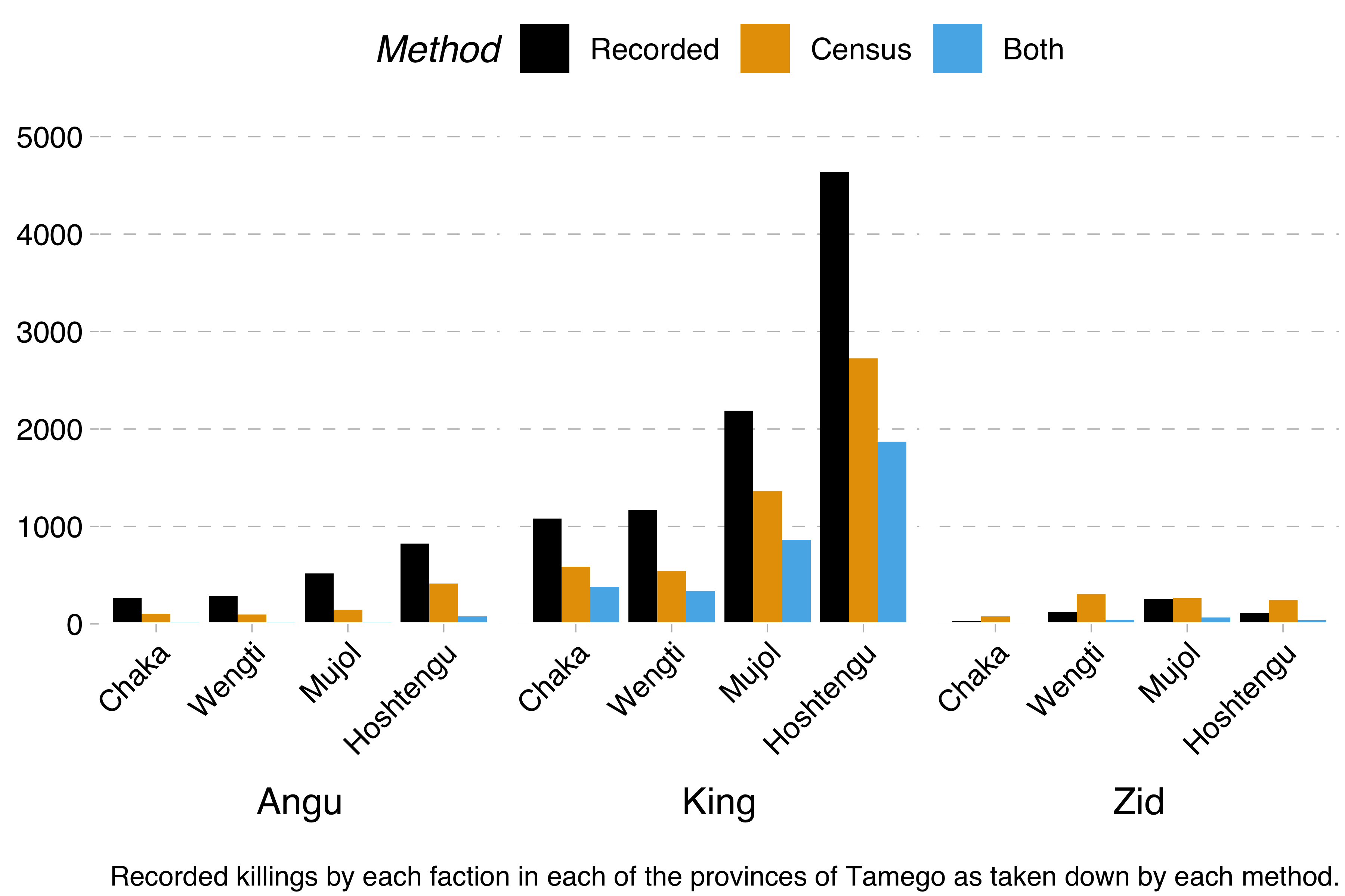
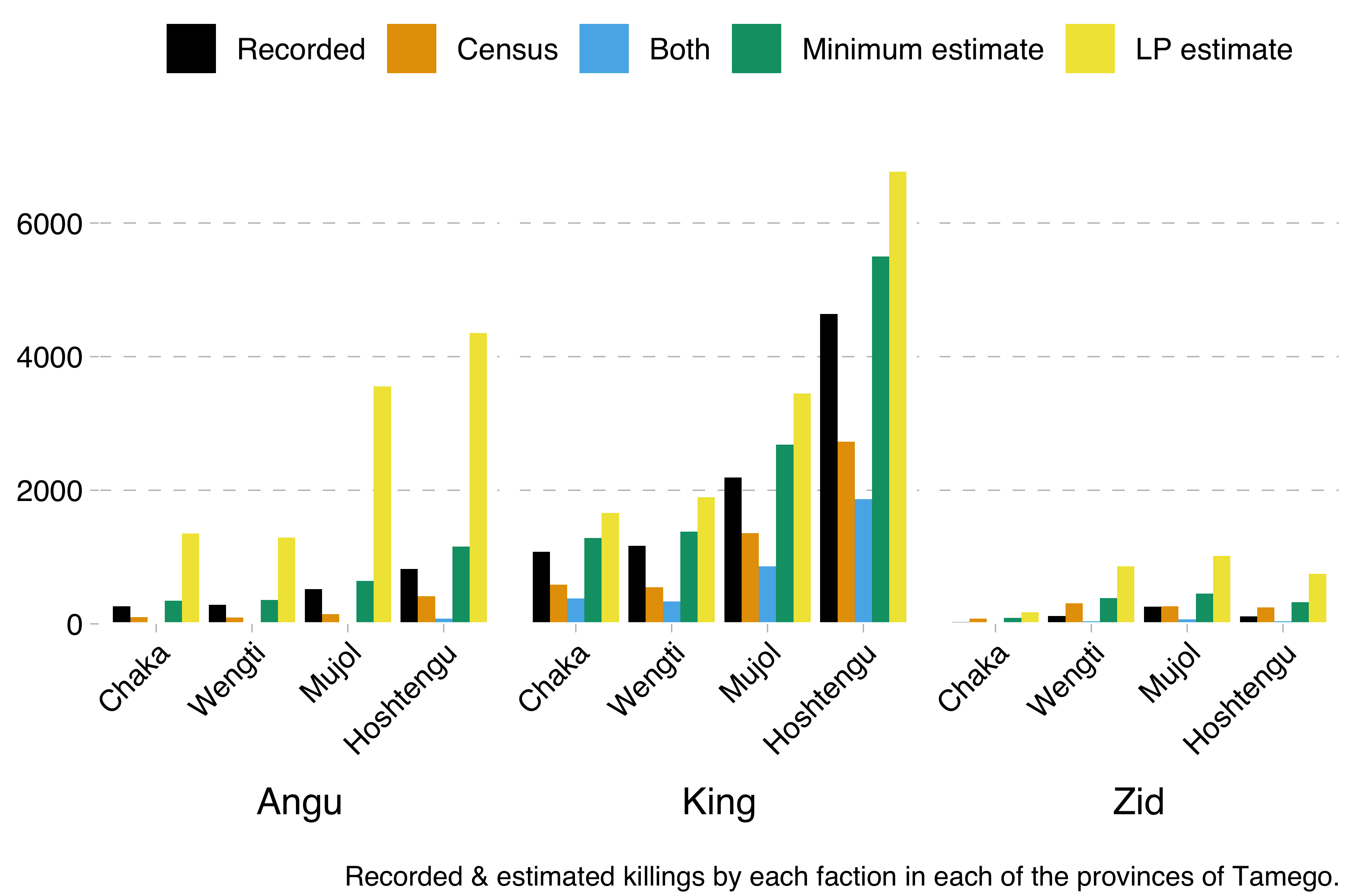
From this data, we were able to calculate the minimum number of killings by each faction and in each region with the formula recorded + census - both. We were also able to calculate Lincoln-Petersen estimates with the formula recorded * census / both.

Now, we could have just encoded that formula in Stan. However, Kéry & Schaub’s model works differently. It uses something called data augmentation (a different sort from the one used to increase training sets in deep learning). The idea here is that you encode the capture-recapture data in a matrix, where each row is one individual and each column one observation (in our case, there would be one column for the official records and one column for the census data). Say for example that we have observed four individuals across two observations. We saw the first individual on both occasions, the second and third only on the first occasion and the fourth only on the second occasion. That would give us this matrix:

1st obs.    2nd obs.
1           1
1           0
1           0
0           1

The trick here is to then add a bunch of additional, unsighted individuals, potential members of the population that we are trying to estimate. This is the data augmentation step. The exact number does not matter, except that it needs to be larger than the population we are trying to estimate. If we knew the population we are estimating was under ten, we could add six unseen individuals:

1st obs.    2nd obs.
1           1
1           0
1           0
0           1
0           0
0           0
0           0
0           0
0           0
0           0

Then, instead of estimating the whole population size N, we recast the problem to one of estimating the inclusion probability omega, that is the probability that any member – sighted or not – in the augmented data set is part of the true population, N. Using this, we can then easily estimate the population. If we find out, for example, that omega_est = .6 in our toy example, it follows that N_est = omega_est * 10 = 6. So the task of the model is to infer omega.

This inference is done for each faction-region combination. But note that there are considerable similarities between the regions. If one faction had larger fighting forces or better military capabilities, for example, they might have killed more in all regions. Or perhaps it is likely that the official military records are biased in such a way that the king’s forces’ killings are better recorded than the rebels’ and separatists’. We can use this fact to our advantage by partially informing the estimate for each faction-region combination using data for the other factions and regions. This is called partial pooling, and it is my addition to Kéry & Schaub’s model (though as it turns out it is not clear whether it actually helps).

Finally we are ready to look at the code. We begin by declaring our input types:

data {
  int<lower=0> P; // number of distinct populations
  int<lower=0> R; // number of distinct regions
  int<lower=0> M; // size of augumented data set
  int<lower=0> T; // number of sampling occasions
  int<lower=0, upper=1> y[P, R, M, T]; // capture-history matrix
}

We then generate some computed variables from that data: the total number of sightings for each faction in each region and in each observation s; and the total number of sighted individuals for each faction in each region C.

transformed data {
  // total number of captures for each potential member
  int<lower=0> s[P, R, M];

  // size of observed data set
  int<lower=0> C[P, R];

  for(i in 1:P) { // for each faction (population)
    for(j in 1:R) { // for each region
      C[i, j] = 0;

      for (k in 1:M) {
        // store the number of captures across all sampling
        // occasions for this potential member.
        s[i, j, k] = sum(y[i, j, k]);

        // if this potential member was observed, increment the
        // count.
        if (s[i, j, k] > 0) {
          C[i, j] = C[i, j] + 1;
        }
      }
    }
  }
}

Then we define the parameters – the unknown variables, those that we are asking Stan to estimate:

parameters {
  // inclusion probability - the probability that any potential member of N
  // (that is, any member of M) is in the true population N
  real<lower=0, upper=1> omega[P, R];

  // detection probability - the probability that any member of N is captured
  vector<lower=0, upper=1>[T] p[P, R];

  real<lower=0, upper=1> p_bar_population[P];
  real<lower=0> sigma_population[P];

  real<lower=0, upper=1> p_bar_region[R];
  real<lower=0> sigma_region[R];
}

Then we define the model:

model {
  // priors are implicitly defined as `uniform(0, 1)'.

  for (i in 1:P) { // for each faction (population)
    for (j in 1:R) { // for each region
      p[i, j] ~ normal(p_bar_population[i], sigma_population[i]);
      p[i, j] ~ normal(p_bar_region[j], sigma_region[j]);

      for (k in 1:M) {
        if (s[i, j, k] > 0) {
          // this potential member was observed, which means it's a member of N.

          // probability that this one is a real member of N
          target += bernoulli_lpmf(1 | omega[i, j]) +
          // probability that this one was sighted during the sampling occasions
            bernoulli_lpmf(y[i, j, k] | p[i, j]);
        } else { // s[i, j, k] == 0
          // this potential member was not observed, which means we don't know
          // if it's a member of N or not.

          // probability that it is a real member but wasn't sighted in any of
          // the sampling occasions
          target += log_sum_exp(bernoulli_lpmf(1 | omega[i, j]) +
                                bernoulli_lpmf(y[i, j, k] | p[i, j]),
          // probability that it's not a real member
                                bernoulli_lpmf(0 | omega[i, j]));
        }
      }
    }
  }
}

And finally we use the estimated inclusion probability, omega, to also estimate the population size N. This is made a little bit tricker because we want to define a different lower bound (the lower bound is the number of individuals known to be sighted in at least one of the observations, calculated with recorded + census - both) for each faction-region combination, which is not possible in Stan. Instead we have to calculate the number of additional individuals beyond the minimum amount (with a fixed lower bound of zero) and after that add the minimum amount to this estimate.

generated quantities {
  // because stan does not support vectors where each element has a different
  // upper/lower constaint, we need to calculate the population size as scaled
  // to (0, 1) and then rescale it.
  //
  // => https://mc-stan.org/docs/2_18/stan-users-guide/vectors-with-varying-bounds.html
  real<lower=0, upper=1> N_raw[P, R];
  real<lower=0, upper=M> N[P, R];

  for (i in 1:P) { // for each faction (population)
    for (j in 1:R) { // for each region
      // calculate the population size.

      // probability of a member, real or not, not being sighted across all
      // sampling occasions.
      real pr = prod(1 - p[i, j]);

      // `omega_nd' is the probability that a potential member is real given it
      // was never detected.

      // probability of a member being real but not being sighted across all
      // sampling occasions.
      real omega_nd = (omega[i, j] * pr) /
        // probability of a member, real or not, not being sighted across all
        // sampling occasions.
        (omega[i, j] * pr + (1 - omega[i, j]));

      // calculate the estimated population size minus the known minimum, scaled
      // to (0, 1).
      N_raw[i, j] = binomial_rng(M - C[i, j], omega_nd) * 1.0 / (M - C[i, j]);

      // rescale the estimated population size minus the known minimum, then add
      // the known minimum to produce the final estimate.
      N[i, j] = N_raw[i, j] * (M - C[i, j]) + C[i, j];
    }
  }
}

So what happens if we run this model using the Kingdom of Tamego data? This happens:

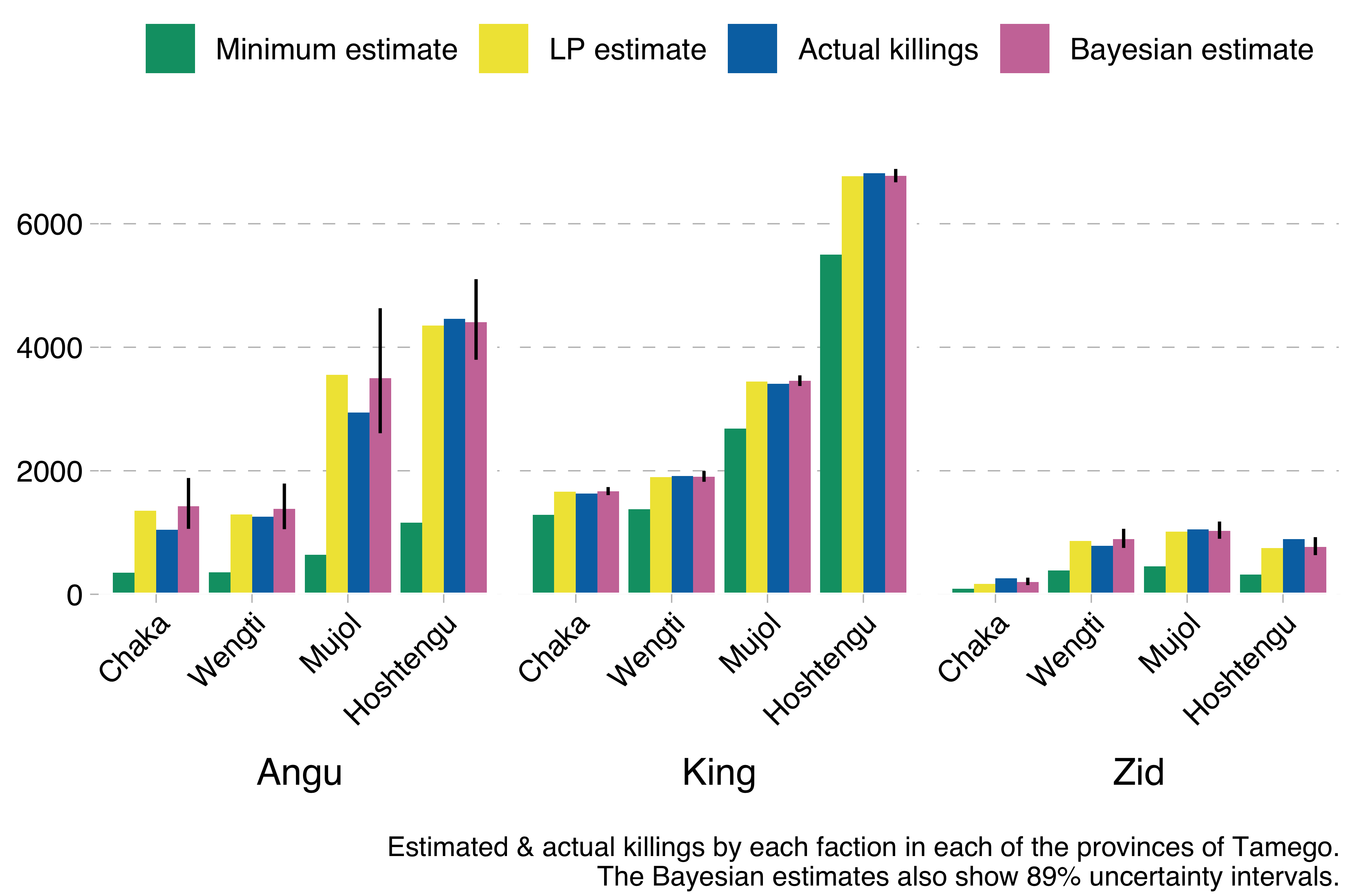
The model produces results basically identical to the much simpler Lincoln-Petersen estimates, but with the additional advantage of allowing us to compute uncertainty intervals. In the graph above I show 89% uncertainty intervals for the Bayesian estimate (the vertical line). These are much wider for the Angu rebel estimates, indicating that mean estimates for that faction are less reliable than for the other factions, which we also know to be true, because we have simulated the data and can see how far off the estimates are from the true values.

This is not a novel use of the capture-recapture method. It has previously been employed to estimate the number of Gulf War veterans who have ALS^[2]; opioid use in Massachusetts^[3]; software defects^[4]; traffic injuries and deaths in Karachi^[5]; and, indeed, killings in the internal conflict in Peru^[6][7][8][9] among much else. This is in addition to its extensive use in population ecology. It is, in other words, an established method, to which I am not sure whether partially pooling faction- and region-level data actually adds anything; in future, I might use Hiroki Itô’s original model to make estimations on the same data and compare the results with my extended model. But even if my extension is not an improvement on the original, simpler model, doing this exercise has taught me a lot about population ecology, R, Stan and good Bayesian modelling workflows, which was the goal in any case.

I will end by observing that the model makes a number of assumptions. One of those assumptions is that the numbers of individuals whose names appear in both the official records and the census need to be large enough that the estimates are not noisy. The model will not capture uncertainty correctly if that is the case – it will be fairly confident yet utterly wrong. This will be the subject of the next and final post in this series.

You can find the code for the model here, though it is kind of messy and I am too exhausted with it all to summon the willpower to clean it up.

Footnotes #

1. Here is the thread in question; thanks go to Ara Winter, Max Joseph, Jacob Socolar and Michael Betancourt for helping me debug issues, pointing me to resources and explaining stuff. ↩︎

2. Coffman, C. J., Horner, R. D., Grambow, S. C., & Lindquist, J. (2005). Estimating the Occurrence of Amyotrophic Lateral Sclerosis among Gulf War (1990–1991) Veterans Using Capture-Recapture Methods. Neuroepidemiology, 24(3), 141–150. ↩︎

3. Barocas, J. A., White, L. F., Wang, J., Walley, A. Y., LaRochelle, M. R., Bernson, D., Land, T., Morgan, J. R., Samet, J. H., & Linas, B. P. (2018). Estimated Prevalence of Opioid Use Disorder in Massachusetts, 2011–2015: A Capture–Recapture Analysis. American Journal of Public Health, 108(12), 1675–1681. ↩︎

4. Briand, L. C., El Emam, K., Freimut, B. G., & Laitenberger, O. (2000). A comprehensive evaluation of capture-recapture models for estimating software defect content. IEEE Transactions on Software Engineering, 26(6), 518–540. ↩︎

5. Razzak, J. (1998). Estimating deaths and injuries due to road traffic accidents in Karachi, Pakistan, through the capture-recapture method. International Journal of Epidemiology, 27(5), 866–870. ↩︎

6. Manrique-Vallier, D., Ball, P., & Sulmont, D. (2019). Estimating the Number of Fatal Victims of the Peruvian Internal Armed Conflict, 1980-2000: an application of modern multi-list Capture-Recapture techniques. arXiv preprint arXiv:1906.04763. ↩︎

7. Rendon, S. (2019). Capturing correctly: A reanalysis of the indirect capture–recapture methods in the Peruvian Truth and Reconciliation Commission. Research & Politics, 6(1), 2053168018820375. ↩︎

8. Manrique-Vallier, D., & Ball, P. (2019). Reality and risk: A refutation of S. Rendón’s analysis of the Peruvian Truth and Reconciliation Commission’s conflict mortality study. Research & Politics, 6(1), 2053168019835628. ↩︎

9. Rendon, S. (2019). A truth commission did not tell the truth: A rejoinder to Manrique-Vallier and Ball. Research & Politics, 6(2), 2053168019840972. ↩︎

Like this post? Subscribe via RSS or join the email newsletter: